| $A$2 | The column and the row do not change when copied. |
|---|---|
| A$2 | The row does not change when copied. |
| $A2 | The column does not change when copied. |
Overall Goals
- Into to Text Mining
- Keyword searches in Excel
- Getting started with R
- Text mining in R
- Text mining in Python
Poll
- What do you think of when I say text mining?
- How much experience do you have with coding languages like R or Python?
- What types of things are you most interested in? (keywords, sentiment, ngrams, word clouds…)
Intro to Text Mining
What is text mining?
Text mining is the process of extracting information and insights from unstructured text.
Terms to Know
- Natural Language: A natural language, as opposed to an artificially created language such as R or Python, develops gradually and often without thought, over time. (Examples include English or Italian.)
- Natural Language Processing (NLP): refers to the creation and use of computational power in order to process content in natural language.
Terms to Know
- Segmentation/Tokenization: the process of splitting apart pieces of language. Sentence segmentation is the process of breaking sentences apart using tokenizers to examine punctuation, abbreviations, and capitalization. Word tokenization involves breaking out the individual words of a sentence.
Terms to Know
- Text Normalization: involves standardizing text prior to analysis. Examples include the expansion of contractions (don’t -> do not), removal of stop words (of, and, it), correcting misspellings, and stemming (if required)
Terms to Know
- Term Frequency: measures how often a term appears in a document.
- Document Frequency: measures how often a term appears in a corpus of documents.
Terms to Know
- Inverse Document Frequency: a number computed by dividing the total number of documents in the corpus by the number of documents containing the target term and applying a log scale.
- TF-IDF: “Term Frequency-Inverse Document Frequency”. Higher term frequency and a lower document frequency leads to a higher TF-IDF.
Levels of Analysis
- Lexical Analysis: The most basic form of NLP, lexical analysis is focused on analyzing individual words.
- Syntactic Analysis: concerned with processing the grammar of written words.
- Semantic Analysis: builds on lexical and syntactic analyses in order to understand the meanings of words.
- Discourse Analysis: Understanding inferences in language is the domain of discourse analysis.
Choosing a Tool
- Experience: what do you know best?
- Availability: what do you have access to?
- Support: where can you turn when you have problems?
- Longevity: if you win the lottery tomorrow can someone take over?
Excel
Excel Agenda
- Pros and Cons
- Formulas
- Using ChatGPT to help with formulas
- Keyword Search
- Word Count
Pros and Cons
Pros - Universally available - Not going anywhere - Low barrier to entry - Scales in complexity
:::
:::
Cons - Can be difficult to reproduce - Potentially destructive - Doesn’t scale well - Limited options for text mining
:::
::::
Formula: vlookup
=VLOOKUP(Value to look up, Range to look for value, Column for the return value, Type of match)
=VLOOKUP(A1, Lookup!A1:B7, 2, TRUE)
Formula: absolute/relative references
Relative references can move.
A1
Absolute references can’t move.
$A$1
Formula: absolute/relative references
Formula: countif
=COUNTIF(Where are we looking?, What are we looking for?)
=COUNTIF(A:A, “Washington”)
ChatGPT for Formula Help
Warning
Assume that everything you put into ChatGPT (or other LLMs) is public. Do not enter confidential or proprietary information into it.
Tell ChatGPT what is is you need assistance with:

ChatGPT for Formula Help
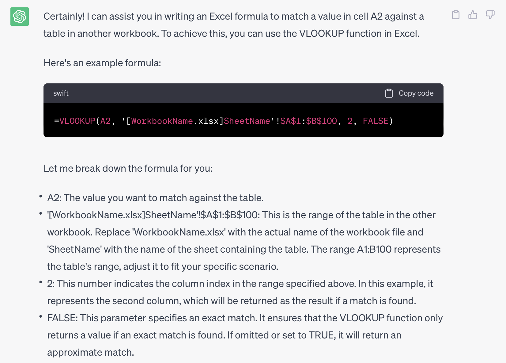
Formula: keyword search
Source: ChatGPT
=IF(SUMPRODUCT(–ISNUMBER(SEARCH(Keywords_Range, Cell)))>0, “Found”, “Not Found”)
Formula: keyword search
=IF(SUMPRODUCT(–ISNUMBER(SEARCH(Keywords_Range, Cell)))>0, “Found”, “Not Found”)
- Replace
Keywords_Rangewith the actual range of keywords you want to search for. For example, if your keywords are in cells A1 to A10, the range would beA1:A10.
Formula: keyword search
=IF(SUMPRODUCT(–ISNUMBER(SEARCH(Keywords_Range, Cell)))>0, “Found”, “Not Found”)
- Replace
Cellwith the cell reference of the cell in the column you want to search. This is the cell where you want to check if any of the keywords are present. For example, if you want to search in column B, and the first cell is B2, you would useB2as the cell reference.
Formula: keyword search
Source: ChatGPT
=IF(SUMPRODUCT(–ISNUMBER(SEARCH(Keywords_Range, Cell)))>0, “Found”, “Not Found”)
- Enter the formula in the cell where you want the search result to appear.
The formula will return “Found” if any of the keywords in the range are found in the specified cell, and “Not Found” if none of the keywords are found.
Note: This formula is case-insensitive, so it will match keywords regardless of their case. If you want case-sensitive matching, you can use the FIND function instead of SEARCH in the formula.
R
Getting Started
- What is R?
- R vs. Python?
Getting Started
Tip
Everything in this workshop can be done through the virtual project. Scan the QR code to get started.

RStudio IDE/Posit Cloud
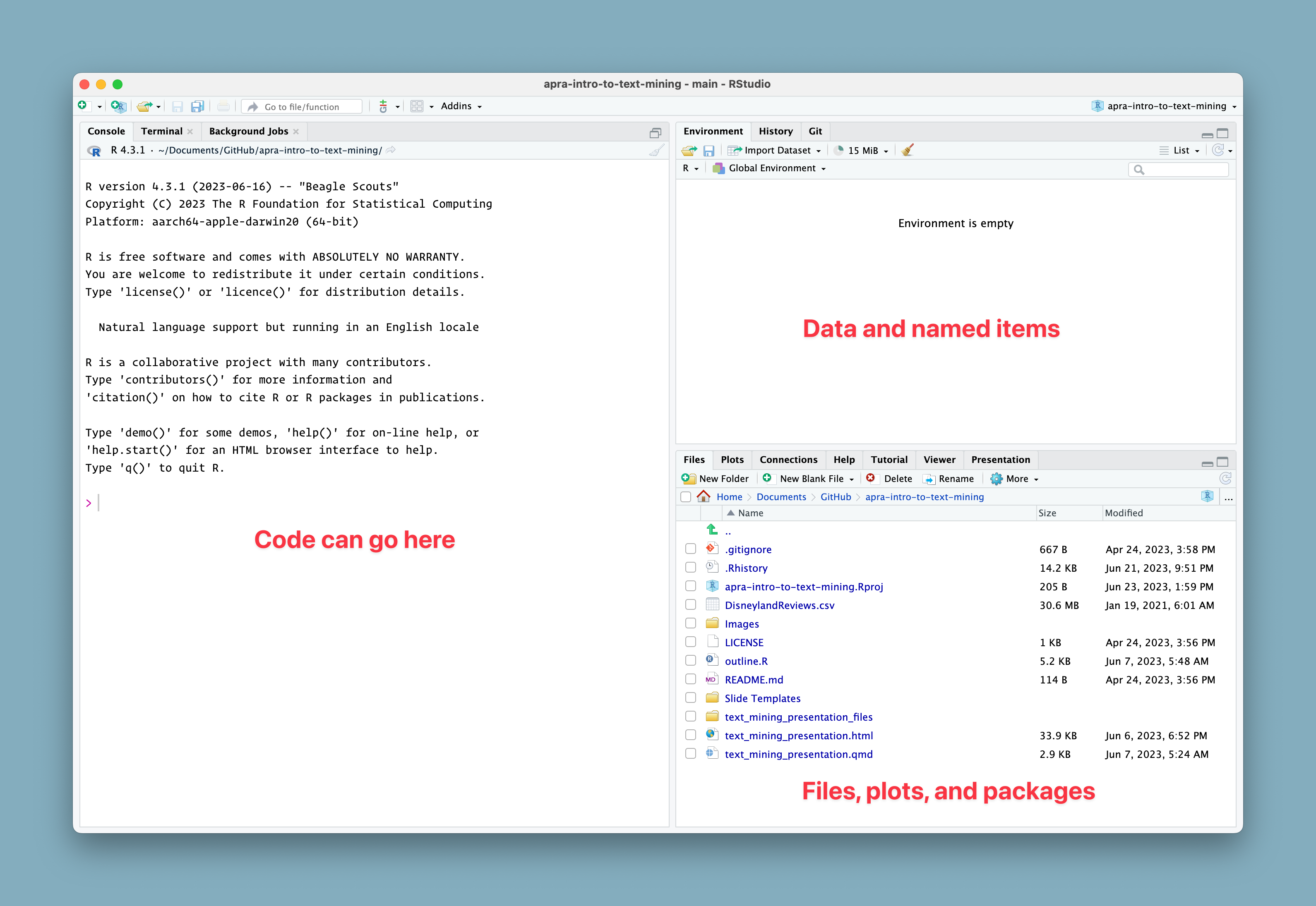
RStudio IDE/Posit Cloud
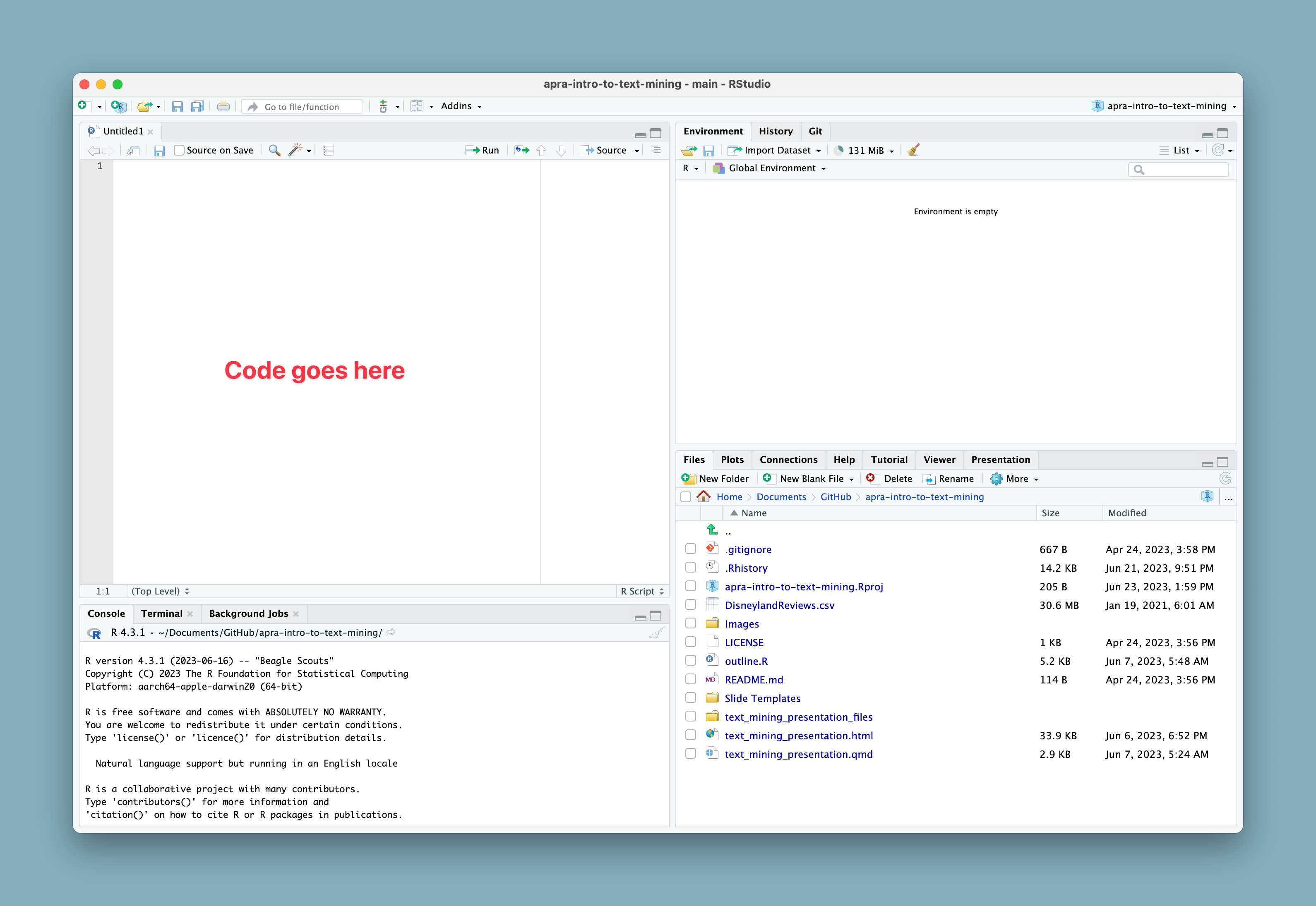
Packages
- Libraries of code
- Expand the “base R” code
The tidyverse

- What is it?
- How does it work?
The tidyverse vs ‘Base R’
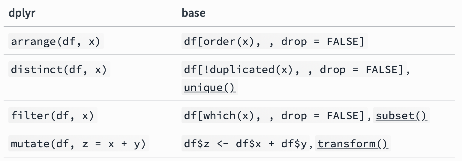
Source: dplyr base R
tidytext

- What is it?
- How does it work?
The Data
42,656 reviews from Disney California, Hong Kong, and Paris

Source: Kaggle
Getting Started
Examine the Data
Rows: 42,656
Columns: 6
$ Review_ID         <dbl> 670772142, 670682799, 670623270, 670607911, 67060729…
$ Rating            <dbl> 4, 4, 4, 4, 4, 3, 5, 3, 2, 5, 5, 5, 4, 5, 5, 3, 4, 3…
$ Year_Month        <chr> "2019-4", "2019-5", "2019-4", "2019-4", "2019-4", "2…
$ Reviewer_Location <chr> "Australia", "Philippines", "United Arab Emirates", …
$ Review_Text       <chr> "If you've ever been to Disneyland anywhere you'll f…
$ Branch            <chr> "Disneyland_HongKong", "Disneyland_HongKong", "Disne…
Look at the Parks
Clean up Park Names
Examine the Data
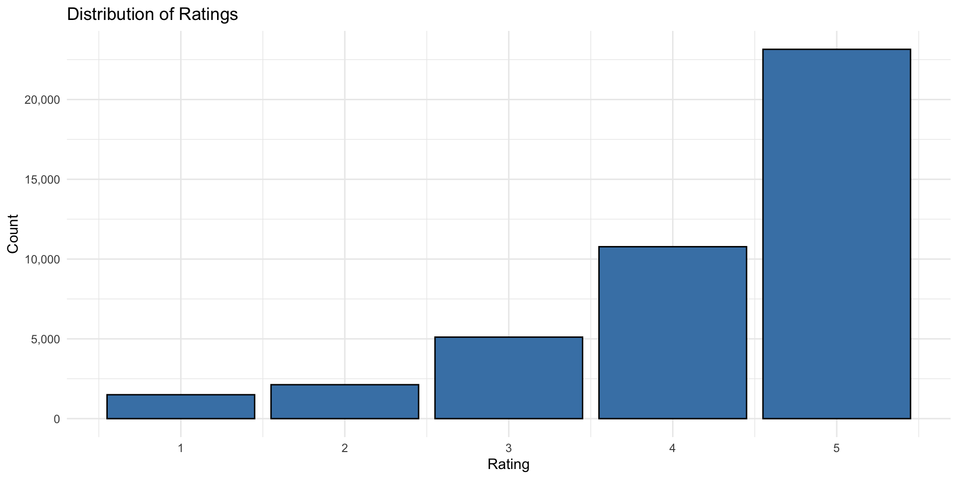
Examine the Data
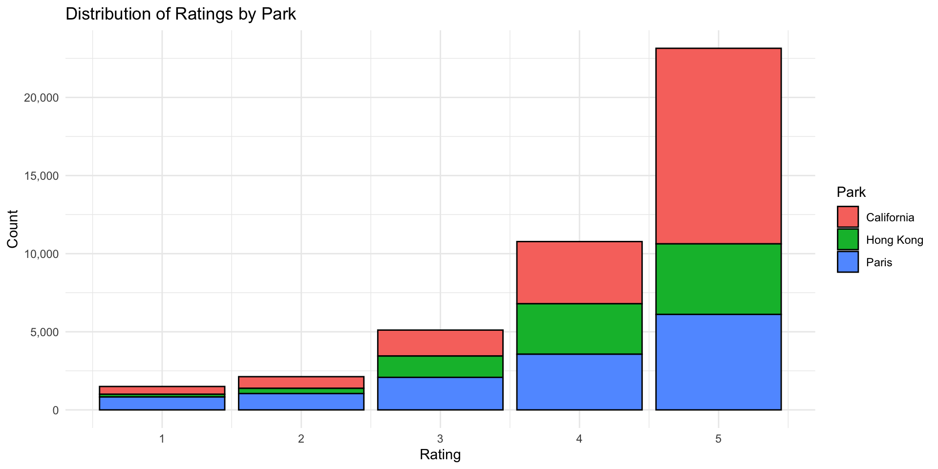
Examine the Data
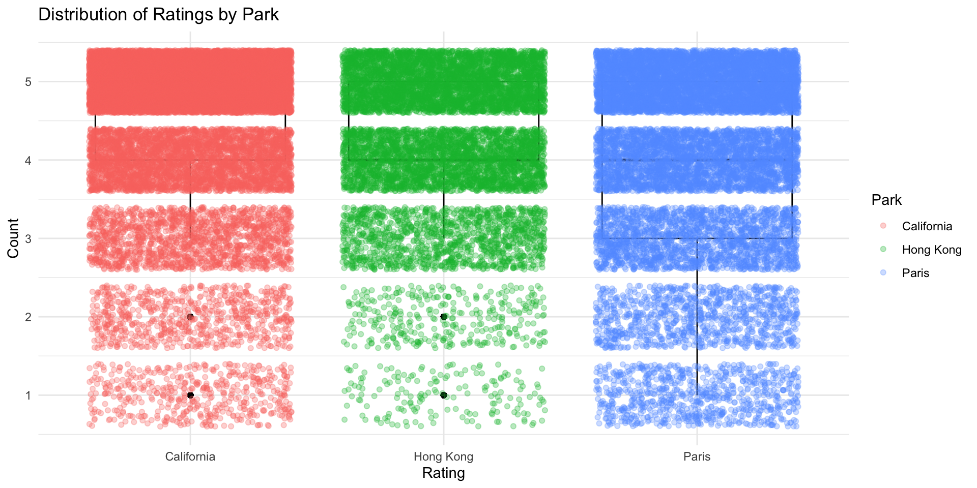
Sample Data
Sample Review
[1] "This place is HUGE! Definately need more than one day. We had 3 children aged 11, 9 & 6 and they loved it. A great variety of rides and attractions for all ages. Food options were fantastic with 3D models of what you were ordering. Staff were fantastic, very helpful. An awesome family experience."Sample Review
# A tibble: 1 × 2
   line text
  <dbl> <chr>
1     1 This place is HUGE! Definately need more than one day. We had 3 childre…
Sample Review: Unnest Tokens
# A tibble: 53 × 2
    line word
   <dbl> <chr>
 1     1 this
 2     1 place
 3     1 is
 4     1 huge
 5     1 definately
 6     1 need
 7     1 more
 8     1 than
 9     1 one
10     1 day
# ℹ 43 more rows
Sample Review: Word Count
# A tibble: 6 × 2
  word          n
  <chr>     <int>
1 were          3
2 and           2
3 fantastic     2
4 of            2
5 11            1
6 3             1
Sample Review: Word Count w/o Stop Words
# A tibble: 6 × 2
  word          n
  <chr>     <int>
1 fantastic     2
2 11            1
3 3             1
4 3d            1
5 6             1
6 9             1
Processing the Data
Number Each Review
# A tibble: 6 × 3
  Park       linenumber text
  <chr>           <int> <chr>
1 California          1 This place has always been and forever will be special.…
2 California          2 A great day of simple fun and thrills. Bring cash, noth…
3 California          3 All and all a great day was had. The crowds are huge an…
4 California          4 Having been to the Florida location numerous times over…
5 California          5 Had the 4 day pass, spent 3 at DL and one at CA. Great …
6 California          6 Oh my god you can really forget your self and enjoy eve…
Unnest Tokens & Remove Stop Words
# A tibble: 6 × 3
  Park       linenumber word
  <chr>           <int> <chr>
1 California          1 forever
2 California          1 special
3 California          1 feeling
4 California          1 entering
5 California          1 park
6 California          1 characters
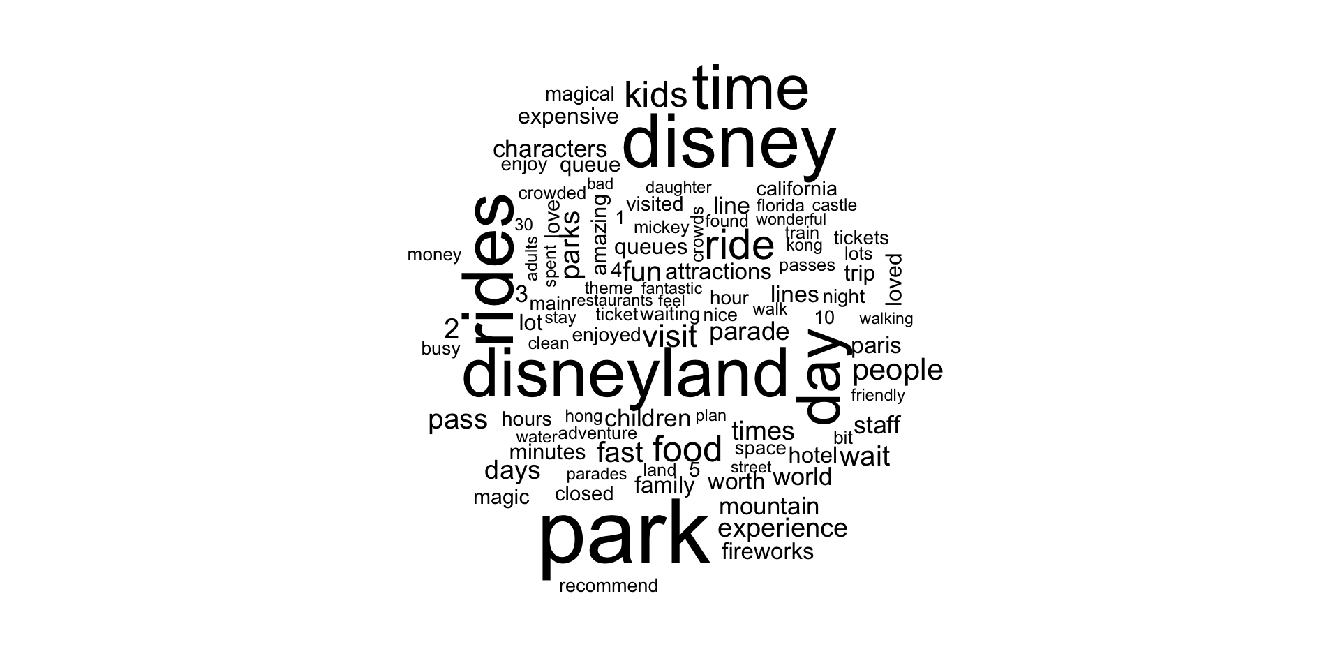
Word Counts
# A tibble: 6 × 2
  word           n
  <chr>      <int>
1 park       44557
2 disney     36187
3 rides      34508
4 disneyland 32935
5 time       29432
6 day        28332
Word Clouds
N-Grams
- A continuous sequence of
nwords - Can be used ‘as is’, or run through a stemmer to get morphemes
- Offers greater context than single words
Bigrams (prep)
# Unnest into bigrams
tidy_bigrams <- reviews %>%
  unnest_tokens(bigram, text, token = "ngrams", n = 2) %>%
  filter(!is.na(bigram))

# Separate words
tidy_bigrams <- tidy_bigrams %>%
  separate(bigram, c("word1", "word2"), sep = " ")

# Remove stop words
tidy_bigrams <- tidy_bigrams %>%
  filter(!word1 %in% stop_words$word) %>%
  filter(!word2 %in% stop_words$word)

# Reunite terms
tidy_bigrams <- tidy_bigrams %>%
  unite(bigram, word1, word2, sep = " ")
Bigrams
# A tibble: 6 × 3
# Groups:   Park [3]
  Park       bigram                   n
  <chr>      <chr>                <int>
1 California fast pass             3123
2 Hong Kong  hong kong             3025
3 Paris      disneyland paris      2932
4 California california adventure  2293
5 Paris      fast pass             1940
6 California disney world          1926
Word & Document Frequencies
Sentiment Analysis
An introduction using the ‘joy’ sentiment.
# A tibble: 6 × 2
  word          sentiment
  <chr>         <chr>
1 absolution    joy
2 abundance     joy
3 abundant      joy
4 accolade      joy
5 accompaniment joy
6 accomplish    joy
Sentiment Analysis
# A tibble: 6 × 2
  word        n
  <chr>   <int>
1 food    14322
2 fun      9952
3 parade   8468
4 love     5967
5 magical  5190
6 enjoy    4807
Sentiment Analysis
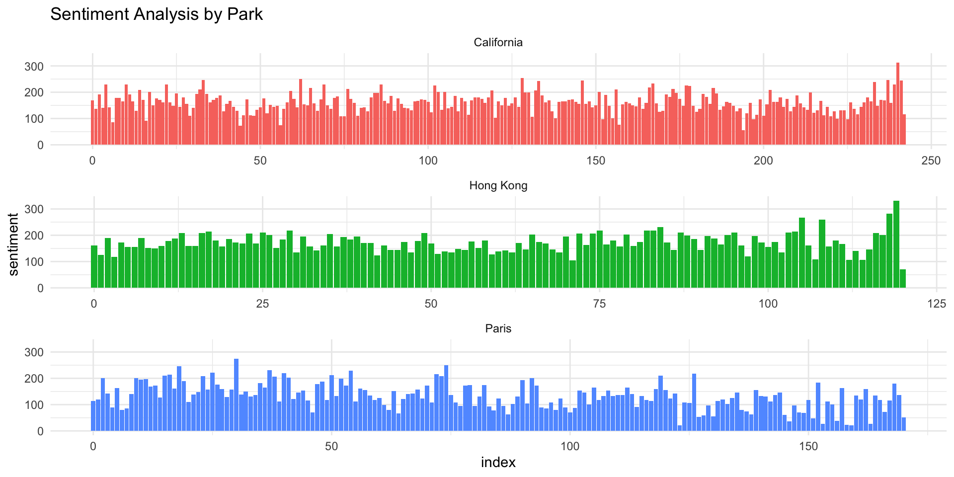
# A tibble: 6 × 5
  Park       index negative positive sentiment
  <chr>      <dbl>    <int>    <int>     <int>
1 California     0      144      313       169
2 California     1      174      310       136
3 California     2      149      340       191
4 California     3      143      283       140
5 California     4      170      399       229
6 California     5      123      266       143
Sentiment Analysis
Topic Modeling
Python
Python Libraries
Recreating R Work
Learning More
Related to this Workshop
Other R Links
Get in Touch
matt.farrow@childrens.com